For those of you who are interested in calculating marine CO₂ system variables, we are happy to let you know that propagating uncertainty in these calculations just got easier. IAEA Ocean Acidification International Coordination Centre (OA-ICC) funded an effort to code a consistent set of tools in several public packages. Uncertainty propagation add-ons are now available for four of these packages: CO2SYS-Excel, CO2SYS-MATLAB, seacarb, and mocsy. Clicking on those links will lead you directly to the archive where each package can be downloaded, on CRAN for seacarb and on GitHub for the other 3 packages.  Links to the uncertainty propagation add-ons can also be found on our Standards and Methods site. A new publication detailing this effort, the tools, and interpretation of results is now available (Orr et al., 2018). The authors highlight, among other things, the use of a new error-space diagram to assess how propagated uncertainty changes with different input uncertainties. The paper also concludes that uncertainties from the constants often dominate propagated uncertainty, so that measurement uncertainty plays little role.

About the tools:

From Jim Orr's blog on ocean carbon science:

"The interface for the CO2SYS-Excel add-on is provided in the same file as the standard package but as an additional (fourth) Excel sheet, where input uncertainties (standard uncertainties) are entered and where calculated uncertainties (combined standard uncertainties) are displayed (after clicking the red START button on Sheet 3). For the add-ons to the other three packages, each is provided as a new routine called errors with a suffix that depends on the computer language of each package (.m, .R, and .f90). Its arguments are just like those for the preexisting routine in each package that computes carbonate chemistry variables (CO2SYS.m, carb.R, and vars.f90, respectively) except that there is also a new line of arguments for the input uncertainties. Besides the typical documentation for each package, the new archives for CO2SYS-MATLAB, seacarb, and mocsy also contain a notebooks directory, which itself contains jupyter notebook files with extensive examples. Once in that directory, just click on a notebook file to visualize its contents as HTML. Even better, download them and and run them interactively in your browser as jupyternotebooks."

The error-space diagram:

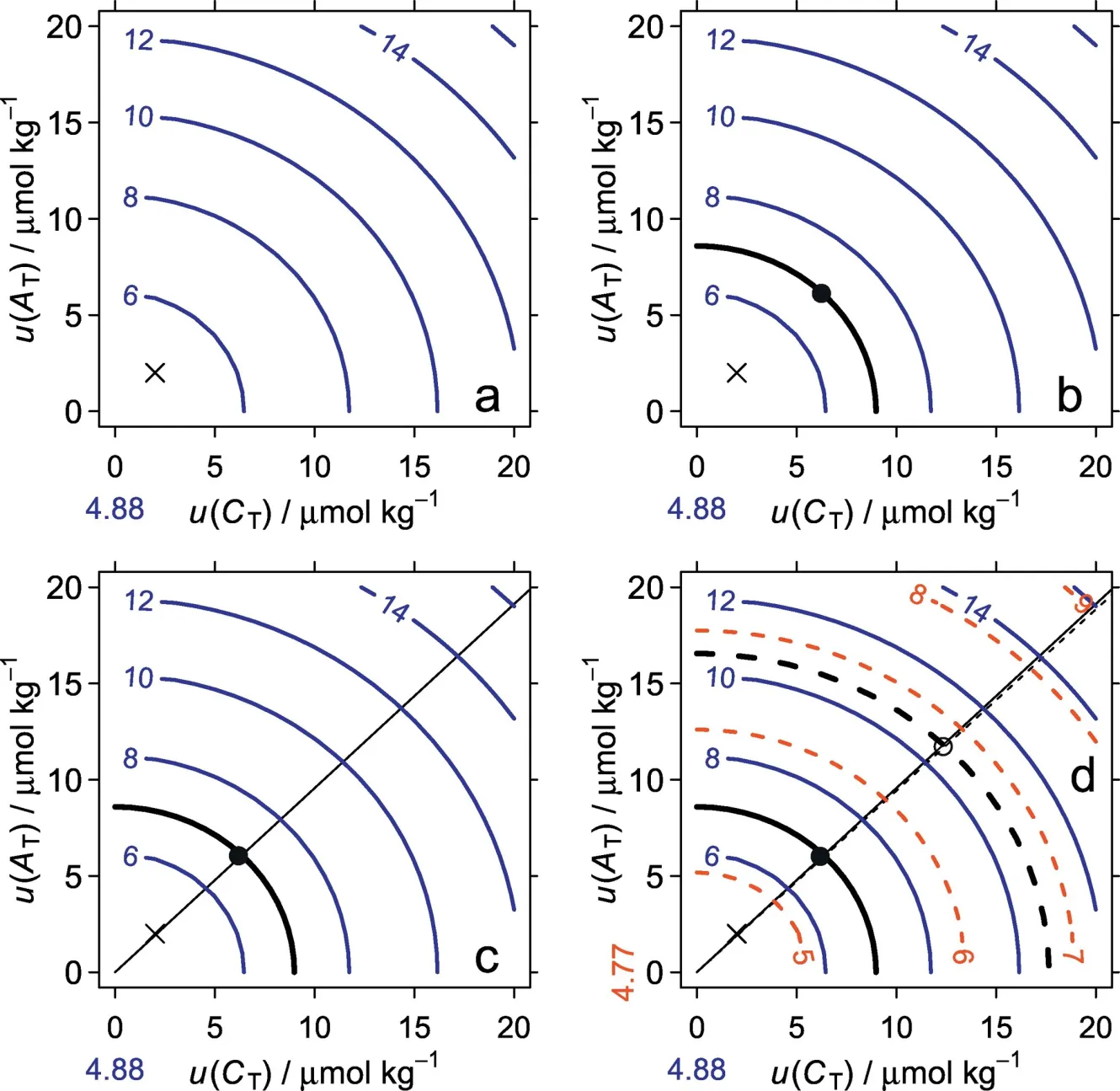
Below is an example of how this new type of diagram, the error-space diagram, looks like. It illustrates how changes in standard uncertainties of a chosen input pair affect a derived variable's combined standard uncertainty. Thus, it is analogous to the more conventional diagram where contours of a derived variable (e.g., pCO₂) are shown as a function of the two members of an input pair (e.g., AT and CT) except that the axes and contours are the uncertainties. See the reference below for a complete anatomy of this diagram, including the exact description of this example as Figure 2 in the paper.

Reference:

Orr, J. C., Epitalon, J.-M., Dickson, A. G., and Gattuso, J.-P. Routine uncertainty propagation for the marine carbon dioxide system, Mar. Chem., 207, 84-107, doi:10.1016/j.marchem.2018.10.006, 2018.